Solving a Laplace problem with Dirichlet boundary conditions
Background
In this tutorial we will solve a simple Laplace problem inside the unit sphere \(\Omega\) with Dirichlet boundary conditions. The PDE is given by
in \(\Omega\) with boundary conditions
on the boundary \(\Gamma\) of \(\Omega\). The boundary data is a source \(\hat{u}\) located at the point \((.9,0,0)\).
For this example we will use an direct integral equation of the first kind. Let
the Green’s function in three dimensions with \(|\mathbf x|^2=x^2+y^2+z^2\). Then from Green’s representation theorem it follows that every function \(u\) harmonic in \(\Omega\) satisfies
Taking the limit \(\mathbf x\rightarrow \Gamma\) we obtain the boundary integral equation
Here, \(V\) and \(K\) are the single and double-layer potential boundary operators defined by
for \(x\in\Gamma\).
Implementation
In the following we demonstrate how to solve this problem with BEM++. We first define the known Dirichlet boundary data. In this example we will use a Python function for it. Other ways are possible (such as a vector of coefficients at the nodes of a mesh).
import numpy as np
def dirichlet_data(x,n,domain_index,result):
    result[0] = np.log(((x[0]-.9)**2+x[1]**2+x[2]**2)**(0.5))
A valid Python function to define a BEM++ GridFunction takes the inputs
x,n,domain_index and result. x is a three
dimensional coordinate vector. n is the normal direction. The
domain_index allows to identify different parts of a physical mesh
in order to specify different functions on different subdomains.
result is a Numpy array that will store the result of the function
call. For scalar problems it just has one component result[0].
We now define a mesh or grid in BEM++ notation. Normally one reads a
grid from a file. BEM++ supports import and export to Gmsh with other
data formats to follow soon. However, for this problem we do not need a
complicated mesh but will rather use the built-in function
grid_from_sphere that defines a simple spherical grid.
from bempp import grid_from_sphere
from bempp.file_interfaces import gmsh
grid = gmsh.GmshInterface("../../meshes/sphere-h-0.1.msh").grid
In order to check how many elements the mesh has we can use the following command
print(grid.leaf_view.entity_count(0))
2570
BEM++ uses Dune-Grid for its Grid management and the principle layout of a Dune grid is accessible from Python via the BEM++ library.
We now define the spaces. For this example we will use two spaces, the space of continuous, piecewise linear functions and the space of piecewise constant functions. The space of piecewise constant functions has the right smoothness the unknown Neumann data. We will use continuous, piecewise linear functions to represent the known Dirichlet data.
from bempp import function_space
piecewise_const_space = function_space(grid,"DP",0) # A disccontinuous polynomial ("DP") space of order 0
piecewise_lin_space = function_space(grid,"P",1)    # A continuous piecewise polynomial ("P") space of order 1
We can now define the operators. We need the identity operator, and the single-layer, respectively double-layer, boundary operator. The general calling convention for an operator is
op = factory_function(domain_space,range_space,dual_to_range_space,...)
Typically, for a Galerkin discretisation only the domain space and the dual space (or test space) are needed. BEM++ also requires a notion of the range of the operator. This makes it possible to define operator algebras in BEM++ that can be used almost as if the operators are continuous objects.
from bempp.operators.boundary import sparse
from bempp.operators.boundary import laplace as boundary_laplace
id = sparse.identity(piecewise_lin_space, piecewise_lin_space, piecewise_const_space)
dlp = boundary_laplace.double_layer(piecewise_lin_space, piecewise_lin_space, piecewise_const_space)
slp = boundary_laplace.single_layer(piecewise_const_space, piecewise_lin_space, piecewise_const_space)
We now define the GridFunction object on the sphere grid that represents the Dirichlet data. If we specify a GridFunction using a Python function as input we will need to declare not only a function space, but also its dual in order to compute the projection of the python function onto the space.
from bempp import GridFunction
dirichlet_fun = GridFunction(piecewise_lin_space, dual_space=piecewise_const_space, fun=dirichlet_data)
The below code will assemble the identity and double-layer boundary operator and evaluate the right-hand side of the boundary integral equation. This is an exact analogue of the underlying mathematical formulation. Depending on the grid size this command can take a bit since here the actual operators are assembled. The left-hand side only consists of the single-layer potential operator in this example. This is here not yet assembled as it is not yet needed. In BEM++ operators are only assembled once they are needed.
rhs = (.5*id+dlp)*dirichlet_fun
lhs = slp
We can force the assembly of the lhs operator also using the
command. But this is optional and would otherwise be done at the
beginning of the iterative solver loop.
lhs.weak_form()
<2570x2570 DenseDiscreteBoundaryOperator with dtype=float64>
The following code solves the boundary integral equation iteratively using Conjugate Gradients. BEM++ offers a CG and GMRES algorithm. Internally these are just simple interfaces to the corresponding SciPy functions with the difference that the BEM++ variants accept BEM++ operators and GridFunctions as objects instead of just operators and vectors.
from bempp.linalg.iterative_solvers import cg
neumann_fun,info = cg(slp,rhs,tol=1E-3)
We could have used directly the corresponding SciPy solver using the commands
from scipy.sparse.linalg import cg
sol,info = cg(slp.weak_form(),rhs.projections,tol=1E-3)
neumann_fun = GridFunction(piecewise_const_space,coefficients=sol)
We now want to provide a simple plot of the solution in the (x,y) plane for z=0. First we need to define points at which to plot the solution.
n_grid_points = 150
plot_grid = np.mgrid[-1:1:n_grid_points*1j,-1:1:n_grid_points*1j]
points = np.vstack((plot_grid[0].ravel(),plot_grid[1].ravel(),np.zeros(plot_grid[0].size)))
The variable points now contains in its columns the coordinates of
the evaluation points. We can now use Green’s representation theorem to
evaluate the solution on these points. Note in particular the last line
of the following code. It is a direct implementation of Green’s
representation theorem.
from bempp.operators.potential import laplace as potential_laplace
slp_pot = potential_laplace.single_layer(piecewise_const_space,points)
dlp_pot = potential_laplace.double_layer(piecewise_lin_space,points)
u_evaluated = slp_pot*neumann_fun-dlp_pot*dirichlet_fun
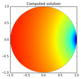
We now want to create a nice plot from the computed data. We only plot a slice through \(z=0\). For a full three dimensional visualization BEM++ allows to export data to Gmsh and VTK.
# The next command ensures that plots are shown within the IPython notebook
%matplotlib inline

# Filter out solution values that are associated with points outside the unit circle.
u_evaluated = u_evaluated.reshape((n_grid_points,n_grid_points))
radius = np.sqrt(plot_grid[0]**2+plot_grid[1]**2)
u_evaluated[radius>1] = np.nan

# Plot the image
import matplotlib
matplotlib.rcParams['figure.figsize'] = (5.0, 4.0) # Adjust the figure size in IPython

from matplotlib import pyplot as plt

plt.imshow(u_evaluated.T,extent=(-1,1,-1,1),origin='lower')
plt.title('Computed solution')
<matplotlib.text.Text at 0x1104733d0>