Grids in BEM++
This tutorial demonstrates basic features of dealing with grids in BEM++. Simple grids can be easily created using built-in commands. More complicated grids can be imported in the Gmsh format.
Creation of basic grid objects
Let us create our first grid, a simple regular sphere.
import bempp.api
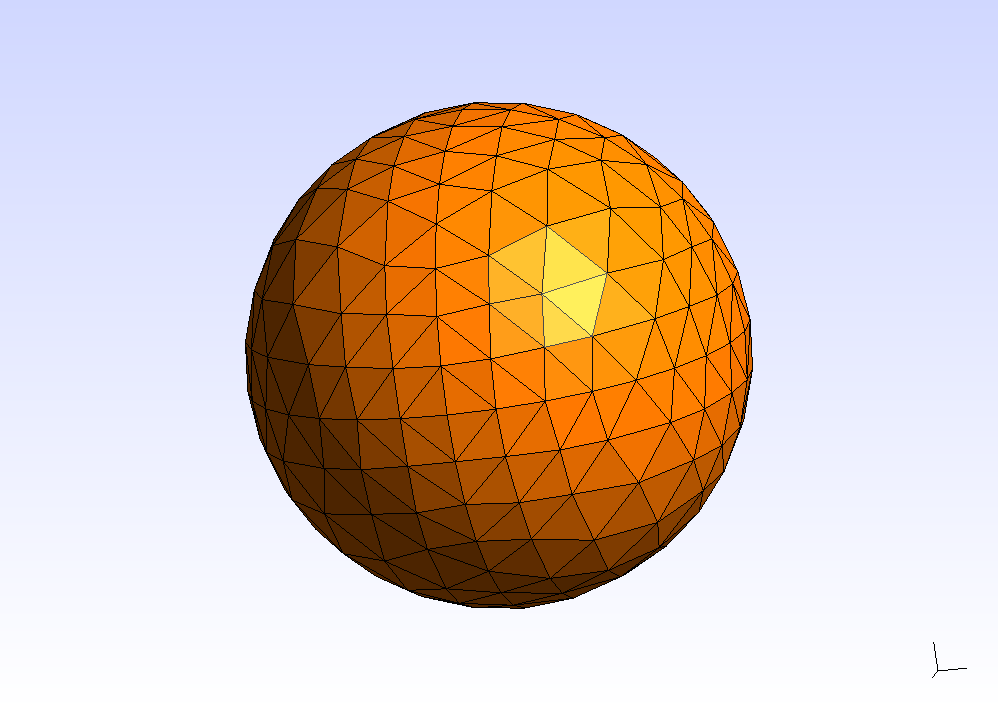
grid = bempp.api.shapes.regular_sphere(3)
The command regular_sphere creates a sphere by refining a base
octahedron. The number of elements in the sphere is given by
nelements = 8 * 4**n, where n is the refinement level. We can
plot the grid with the following command.
grid.plot()
This uses Gmsh to plot the grid externally. In order to work please
make sure that Gmsh is installed and the command gmsh is
available in the path. The following picture shows the sphere.
Another way to create a sphere is by specifying the width of the elements. The command
grid = bempp.api.shapes.sphere(h=0.1)
will create an unstructured spherical grid with a grid size of roughly
0.1. Note that in order for this command to succeed Gmsh as grid
generator must be installed. The shapes module contains functions
for spheres, ellipsoids, cubes and the Nasa almond shape.
Sometimes, it is desired to create a regular structured 2d grid (such as
a screen). For this BEM++ offers the functino
bempp.api.structured_grid. The help text of this function gives more
detail on its use.
Creating grids from connectivity data
Quite often a grid is given in the form of connectivity data, that is an array containing the nodes and another array containing the element defintions from the nodes. Consider the following definition of vertices.
vertices = np.array([[0,1,1,0],
                     [0,0,1,1],
                     [0,0,0,0]])
The array vertices contains the (x,y,z) coordinates of the four
vertices of the unit square in the x-y plane.
We now define two elements by specifiying how the vertices are connected.
elements = np.array([[0,1],
                     [1,2],
                     [3,3]])
The first element connects the vertices 0, 1 and 3. The second element connects the vertices 1, 2 and 3. To create a grid from these two elements we simply call the following command.
grid = bempp.api.grid_from_element_data(vertices,elements)
Please note that BEM++ assumes that each element is defined such that
the normal direction obtained with the right-hand rule is outward
pointing. Elements with inward pointing normals can easily be a source
for errrors in computations. Normal directions can be visually checked
for example by loading a mesh in Gmsh and displaying the normals.
Also, it is not guaranteed that elements are stored in the grid object
using the same numbering as during insertion. Further down we will
explain this in detail. To find out the insertion index of a vertex or
an element the methods grid.vertex_insertion_index and
grid.element_insertion_index are provided.
Importing grids from files
Grids can be imported from external files. BEM++ natively supports the
Gmsh v2.2 msh format (only ASCII and not binary). The Gmsh
documentation gives
details of this format. Gmsh can easily convert from various formats
into .msh. The following command imports a grid into BEM++ from an
external file.
grid = bempp.api.import_grid('my_grid.msh')
Please note that it is important to choose the correct file ending
.msh. BEM++ uses it to recognize the file format.
Iterating through grids
For many BEM++ usage scenarios the internal of the grid object are not important. However, sometimes it may be useful to iterate through a grid and retrieve information from individual elements. Internally, BEM++ uses Dune-Grid to represent a grid. The basic objects in Dune are entities of a given codimension. For surface meshes in BEM++ this translates as follows:
- Codim-0 entities: Elements of the mesh
- Codim-1 entities: Edges of the mesh
- Codim-2 entities: Verticies of the mesh
For example, in order to show the number of elements in the sphere mesh above the following command can be used.
# Create the grid
import bempp.api
grid = bempp.api.shapes.regular_sphere(3)

# Print out the number of elements
number_of_elements = grid.leaf_view.entity_count(0)
print("The grid has {0} elements.".format(number_of_elements))
The grid has 512 elements.
In order to just print out all vertices and elements of a mesh the following commands can be used.
vertices = grid.leaf_view.vertices
elements = grid.leaf_view.elements
We can also iterate through entities and obtain geometric information about them. The following command stores references to all elements in a Python array.
elements = list(grid.leaf_view.entity_iterator(0))
Let us now print out the corners of the first element in this list and the area of the corresponding triangle.
corners = elements[0].geometry.corners
area = elements[0].geometry.volume
print("Corners: {0}".format(corners))
print("Area: {0}".format(area))
Corners: [[ 0.          0.          0.19509032]
 [ 1.          0.98078528  0.98078528]
 [ 0.          0.19509032  0.        ]]
Area: 0.0192138328039
Corners are always interpreted column-wise. Hence, the first corner of
the element is [0, 1, 0]. The volume attribute depends on the
entity. For elements it gives the area and for edges it gives the length
of an edge.
Indexing in Dune is slightly more complicated. The above order from
the iterator is not guaranteed to agree with the internal indices of the
elements. To find out the index of an element or other entity type one
can query an IndexSet object.
index_set = grid.leaf_view.index_set()
index = index_set.entity_index(elements[0])
print("The element index is {0}.".format(index))
The element index is 0.
In this case the index of the first element returned by the iterator is
indeed 0. However, this is dependent on the implementation of the
underlying grid manager and not guaranteed. Furthermore, the indices
from the IndexSet do not need to agree with the order in which
elements and vertices were entered into the grid. However, this
information is often needed to associate given physical data with mesh
entities. For this case the functions grid.element_insertion_index
and grid.vertex_insertion_index are provided. The insertion index of
the first element in the elements list is given as follows.
insertion_index = grid.element_insertion_index(elements[0])
print("Insertion index of first element: {0}.".format(insertion_index))
Insertion index of first element: 0
Again, in this case it agrees with the ordering returned by the
iterator. But this behavior is not guaranteed and indices should always
be computed using an IndexSet or the insertion_index methods.
Factory functions to create grids
The following functions and bempp.api.GridFactory class provide general mechanisms to
create new grids. More specialised routines for certain shapes are also contained in
the module bempp.api.shapes
-
bempp.api.grid_from_element_data(vertices, elements, domain_indices=None)¶ Create a grid from a given set of vertices and elements.
This function takes a list of vertices and a list of elements and returns a grid object.
Parameters: - vertices (np.ndarray[float]) – A (3xN) array of vertices.
- elements (np.ndarray[int]) – A (3xN) array of elements.
Returns: grid – The grid representing the specified element data.
Return type: bempp.Grid
Examples
The following code creates a grid with two elements.
>>> import numpy as np
>>> vertices = np.array([[0,1,1,0],
                         [0,0,1,1],
                         [0,0,0,0]])
>>> elements = np.array([[0,1],
                         [1,2],
                         [3,3]])
>>> grid = grid_from_element_data(vertices,elements)
-
bempp.api.structured_grid(lower_left, upper_right, subdivisions, axis='xy', offset=0)¶ Create a two dimensional rectangular grid.
Parameters: - lower_left (tuple) – The (x,y) coordinate of the lower left corner of the grid.
- upper_right (tuple) – The (x,y) coordinate of the upper right corner of the grid.
- subdivisions (tuple) – A tuple (N,M) specifiying the number of subdivisions in each dimension.
- axis (string) – Possible choices are “xy”, “xz”, “yz”. Denotes the axes along which the structured grid is generated. Default is “xy”.
- offset (double) – Defines an offset value that shifts the structured grid in the remaining coordinate direction.
Returns: grid – A structured grid.
Return type: bempp.Grid
Examples
The following command creates a grid of the unit square [0,1]^2.
>>> grid = structured_grid((0,0),(1,1),(100,100))
-
class
bempp.api.GridFactory¶ Implement a grid factory.
A grid factory can be used to create arbitrary grids from a set of vertices and elements.
Examples
The following gives an example of how to grid an grid containing a single element using a grid factory.
>>> factory = bempp.api.grid.GridFactory()
>>> factory.insert_vertex([0, 0, 0])
>>> factory.insert_vertex([1, 0, 0])
>>> factory.insert_vertex([0, 1, 0])
>>> factory.insert_element([0, 1, 2])
>>> grid = factory.finalize()
-
finalize()¶ Finalize the grid creation and return a grid object.
-
insert_element(element, domain_index=0)¶ Insert an element into a list.
The element must be a list type object with three components specifying the insertion indices of the three vertices associated with the element. The domain_index allows to group elements into different sets with different indicies.
-
insert_vertex(vertex)¶ Insert a vertex into a grid.
The vertex must be a list type object with 3 components.
-
Function and class reference
The following classes define a Grid and its various components. They are not meant to be instantiated directly.