Grid Functions
In BEM++ data on a given grid is represented as a GridFunction
object. A GridFunction consists of a set of basis function
coefficients and a corresponding Space object. In the following we
will discuss the different ways of creating a grid function in BEM++.
Initializing a grid function from a Python callable
Often, in applications we are given an analytic expression for boundary data. This is for example the case in many acoustic scattering problems, where a typical scenario is that the incoming data is a plane wave or a sound source. The following code defines a wave travelling with unit wavenumber along the x-axis in the positive direction.
import numpy as np
def fun(x, normal, domain_index, result):
    result[0] = np.exp(1j * x[0])
A valid Python callable always has the same interface as shown above.
The first argument x is the coordinate of an evaluation point. The
second argument normal is the normal direction at the evaluation
point. The third one is the domain_index. This corresponds to the
physical id in Gmsh and can be used to assign different boundary data to
different parts of the grid. The last argument result is the
variable that stores the value of the callable. It is a numpy array with
as many components as the basis functions of the underlying space have.
If a scalar space is given then result only has one component.
In order to discretise this callable we need to define a suitable space object. Below we define a space of continuous, piecewise linear functions on a spherical grid.
import bempp.api
grid = bempp.api.shapes.regular_sphere(5)
space = bempp.api.function_space(grid, "DP", 1)
The next command now discretizes the Python callable by projecting it onto the space.
grid_fun = bempp.api.GridFunction(space, fun=fun)
There is quite a lot going on now as shown by the output logging
messages. Before we describe in detail what is happening we want to
visualize the grid_fun object. This can be done with the command
grid_fun.plot()
This command opens Gmsh externally as a viewer to show the
GridFunction object. The results should look like the following.
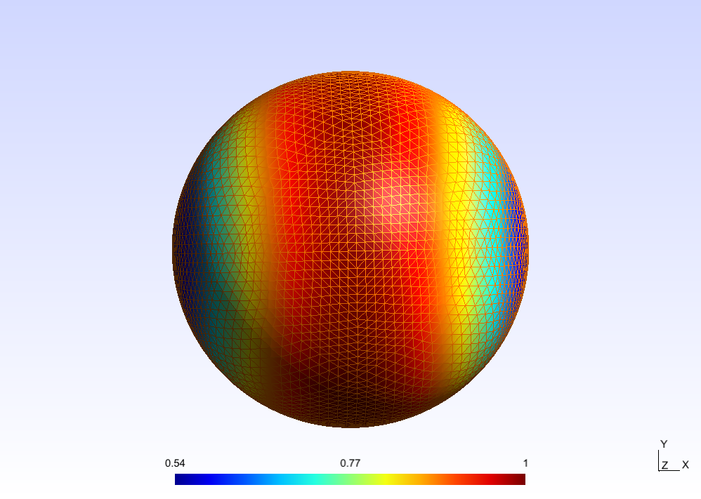
By default the real part of grid_fun is plotted. There are more
advanced functions to control this behavior.
Let us take a closer look at what happens in the initialization of this GridFunction. Denote the global basis functions of the space by \(\Psi_j\), \(j=1,\dots,N\). The computation of the grid function consists of two steps.
- Compute the projection coefficients \(p_j = \int_{\Gamma}\overline{\Psi_j}(\xi)f(\xi)d\xi\), where \(f\) is the analytic function to be converted into a grid function and \(\Gamma\) is the surface defined by the grid.
- Compute the basis coefficients \(c_j\) from \(Mc=p\), where \(M\) is the mass matrix defined by \(M_{ij} = \int_{\Gamma}\overline{\Psi_i}(\xi)\Psi_j(\xi)d\xi\).
This is an orthogonal \(L^2(\Gamma)\)-projection onto the basis given by the \(\Psi_j\).
Initializing a grid function from coefficients or projections
Instead of an analytic expression we can initialize a GridFunction
object also from a vector c of coefficients or a vector p of
projections. This can be done as follows.
grid_fun = GridFunction(space, coefficients=c)
grid_fun = GridFunction(space, projections=p, dual_space=dual)
The argument dual_space gives the space with which the projection
coefficients were computed. The parameter is optional and if it is not
given then space == dual_space is assumed (i.e.
\(L^2(\Gamma)\)-projection).
Function and class reference
-
class
bempp.api.GridFunction(space, dual_space=None, fun=None, coefficients=None, projections=None, parameters=None)¶ Representation of functions on a grid.
-
coefficients¶ np.ndarray – Return or set the vector of coefficients.
-
component_count¶ int – Return the number of components of the grid function values.
-
space¶ bemp.api.space.Space – Return the space over which the GridFunction is defined.
-
grid¶ bempp.api.grid.Grid – Return the underlying grid.
-
parameters¶ bempp.api.ParameterList – Return the set of parameters.
-
representation¶ string – Return ‘primal’ if the coefficients of the Gridfunction are known. Return ‘dual’ if only the coefficients in the dual space are known.
-
coefficients¶ Return the function coefficients.
-
component_count¶ Return the number of components of the grid function values.
-
dtype¶ Return the dtype.
-
dual_space¶ Return the dual space.
-
evaluate(element, local_coordinates)¶ Evaluate grid function on a single element.
-
evaluate_surface_gradient(element, local_coordinates)¶ Evaluate surface gradient of grid function for scalar spaces.
-
classmethod
from_ones(space)¶ Create a grid function with all coefficients set to one.
-
classmethod
from_random(space)¶ Create a random grid function normalized to unit norm.
-
classmethod
from_zeros(space)¶ Create a grid function with all coefficients set to one.
-
grid¶ Return the underlying grid.
-
integrate(element=None)¶ Integrate the function over the grid or a single element.
-
l2_norm(element=None)¶ L^2 norm of the function on a single element or on the mesh.
-
parameters¶ Return the parameters.
-
plot()¶ Plot the grid function.
-
projections(dual_space=None)¶ Compute the vector of projections onto the given dual space.
Parameters: dual_space (bempp.api.space.Space) – A representation of the dual space. If not specified then fun.dual_space is used. Returns: out – A vector of projections onto the dual space. Return type: np.ndarray
-
relative_error(fun, element=None)¶ Relative L^2 error compared to a given analytic function.
Parameters: - fun (callable) – A python callable of the form f(p), where p is a point with the three space components x, y, z at which to evaluate the function.
- element (bempp.api.grid.entity.Entity) – An entity of codimension 0.
-
representation¶ Return ‘dual’ or ‘primal’.
-
space¶ Return the Space object.
-
surface_grad_norm(element=None)¶ Norm of the surface gradient on a single element or on the mesh.
-